Citation:
Yongqiang Li, Yi Xiao, Quan Tao, Mengmeng Yu, Li Zheng, Siwei Yang, Guqiao Ding, Hui Dong, Xiaoming Xie. Selective coordination and localized polarization in graphene quantum dots: Detection of fluoride anions using ultra-low-field NMR relaxometry[J]. Chinese Chemical Letters,
2021, 32(12): 3921-3926.
doi:
10.1016/j.cclet.2021.05.014
Selective coordination and localized polarization in graphene quantum dots: Detection of fluoride anions using ultra-low-field NMR relaxometry
English
Selective coordination and localized polarization in graphene quantum dots: Detection of fluoride anions using ultra-low-field NMR relaxometry
State Key Laboratory of Functional Materials of Informatics, Shanghai Institute of Microsystem and Information Technology, Chinese Academy of Sciences (CAS), Shanghai 200050, China
b.
CAS Center for Excellence in Superconducting Electronics (CENSE), Chinese Academy of Sciences, Shanghai 200050, China
c.
Center of Materials Science and Optoelectronics Engineering, University of Chinese Academy of Sciences, Beijing 100049, China
* Corresponding authors at: State Key Laboratory of Functional Materials of Informatics
Shanghai Institute of Microsystem and Information Technology
Received Date:
21 March 2021 Accepted Date:
13 May 2021 Revised Date:
06 May 2021 Available Online:
15 December 2021
Abstract:
The development of ultra-sensitive methods for detecting anions is limited by their low charge to radius ratios, microenvironment sensitivity, and pH sensitivity. In this paper, a magnetic sensor is devised that exploits the controllable and selective coordination that occurs between a magnetic graphene quantum dot (GQD) and fluoride anion (F–). The sensor is used to measure the change in relaxation time of aqueous solutions of magnetic GQDs in the presence of F‒ using ultra-low-field (118 µT) nuclear magnetic resonance relaxometry. The method was optimized to produce a limit of detection of 10 nmol/L and then applied to quantitatively detect F– in domestic water samples. More importantly, the key factors responsible for the change in relaxation time of the magnetic GQDs in the presence of F‒ are revealed to be the selective coordination that occurs between the GQDs and F‒ as well as the localized polarization of the water protons. This striking finding is not only significant for the development of other magnetic probes for sensing anions but also has important ramifications for the design of contrast agents with enhanced relaxivity for use in magnetic resonance imaging.
The recognition of specific target anions is challenging because of their low charge to radius ratios, microenvironment sensitivity (solvent effect), and pH sensitivity [1]. Structurally, the fluoride anion (F–) has the smallest ionic radius, highest charge density, and weakest Lewis basicity among the inert anions [2], which makes it difficult to be recognized and detected. Therefore, developing effective detection methods for F– is a vitally important step in the development of anion-specific detection procedures and probes.
Some colorimetry-based methods have been investigated for use in F– detection which depend on the identification of certain optical signals [3-5]. In comparison, however, the magnetic signals that are observed in nuclear magnetic resonance (NMR) relaxometry, have the advantage of high penetration depth and are nearly background-free [6, 7]. In recent years, magnetic sensors have been developed to measure the magnetic signals from magnetic probes that have superior properties compared with colorimetry-based detection methods (including enhanced sensitivities and simple methodologies) [8-11]. It is highly likely, therefore, that such methods may allow F‒ to be detected with high sensitivity.
Magnetic lanthanide complexes have been widely adopted as contrast agents in magnetic resonance imaging [12-15]. Lanthanide ions usually contain a large number of unpaired electrons and thus have paramagnetic properties [16]. For example, the gadolinium(Ⅲ) ion (Gd3+) has seven unpaired electrons. Moreover, the symmetric nature of the S-state of the Gd3+ means that it has a much slower electronic relaxation rate that experienced by water protons [17]. Inspired by the fact that colorimetry-based sensors have been devised that exploit the interaction between lanthanide complexes and F‒ [18-20], it can be expected that magnetic sensors should also be realizable that operate in the same way. Despite the fact that lanthanide ions are hard Lewis acids [21], the binding affinities between lanthanide complexes and F– are generally very weak (logKa = 1.5‒3) [22], which means it is difficult to create a lanthanide-based magnetic sensor that can be used to detect F‒ with high sensitivity. Therefore, the crucial issue as far as F‒ detection is concerned to realize a selective and stable interaction between the lanthanide complex employed and the F‒.
Given that graphene quantum dots (GQDs) with modifiable structures [23] and tunable properties [24, 25] can be synthesized in kilogram-scale [26]. In this study, Gd3+-loaded polyethylene glycol (PEG) modified GQDs, hereafter abbreviated as GPGs, are used as magnetic probes to detect F–. In the presence of the PEG with different chain lengths, the F‒ can selectively coordinate with the Gd3+ in the GPGs. The stable coordination of an F‒ to the Gd3+ leads to a strong polarization effect on the bulk water molecules surrounding the GP4G containing tetraethylene glycol (PEG4). This makes the bulk water molecules much more likely to undergo ionization and thus increases the proton exchange rate. These changes in microenvironment are reflected in the longitudinal relaxation time (T1) measured via ultra-low-field (ULF) NMR relaxometry [27].
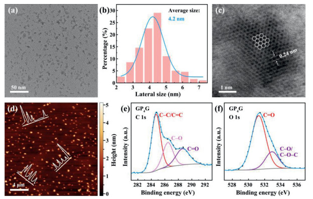
GP4G was obtained using the previously-proposed method (hydrothermal treatment) [14, 28]. Fig. 1 shows the information gathered about the morphology and structure of the GP4G synthesized. The transmission electron microscopy (TEM) image (Fig. 1a) indicates that the GP4G nanoparticles have high dispersibility. The lateral size distribution curve (Fig. 1b) further indicates that the average size of the nanoparticles is 4.2 nm. Fig. 1c is a high-resolution TEM (HR-TEM) image of a GP4G nanoparticle. The image exhibits excellent crystallinity which indicates that the GP4G nanoparticles are well-crystallized. The lattice parameter of 0.24 nm represents the (1120) lattice fringe of graphene. The heights of the GP4G nanoparticles were investigated via atomic force microscope (AFM) on a 300 nm SiO2/Si substrate giving the results shown in Fig. 1d. As can be seen, the heights of the nanoparticles range from 0.5 nm to 1.5 nm corresponding to 1‒4 layers of graphene [29, 30].
Figure 1
Figure 1.
(a) TEM image of GP4G, (b) size distribution histogram (and the corresponding fit to a Gaussian distribution function), and (c) a HR-TEM image of GP4G in which the regular hexagons (white lines) outline the graphene structure. (d) Topographical AFM image of GP4G nanoparticles on a 300 nm SiO2/Si substrate. Inset: height profiles along the lines indicated. The final images are XPS spectra of the GP4G nanoparticles corresponding to (e) C 1s, and (f) O 1s signals.
X-ray photoelectron spectroscopy (XPS) was also used to investigate the chemical structure of the GP4G nanoparticles. An XPS survey spectrum exhibits peaks at 284.8, 531.4, and 142.7 eV which can be attributed to C 1s, O 1s, and Gd 4d signals, respectively (Fig. S1 in Supporting information) [14]. The atomic ratio of C to O in GP4G is found to be 0.9 meaning that it is relatively oxygen-rich. The Gd3+ content of the GP4G is found to be 2.9 at%. The C 1s spectrum of GP4G (Fig. 1e) has peaks located at 284.8, 286.5, and 288.7 eV which can be recognized as C–C/C=C, C–O, and C=O bonds, respectively. The peaks located at 531.3 and 532.9 eV in the O 1s spectrum (Fig. 1f) arise due to C=O and C–O/C–O–C bonds, respectively. The PEG modifies the surface of the GQDs resulting in a high C–O/C–O–C bond content (22.6 at%). Moreover, the Gd3+ combines with the PEG4via a coordination process [14], as shown in Fig. S2 (Supporting information). The X-ray diffraction pattern also confirms the formation of GP4G (Fig. S3 in Supporting information).
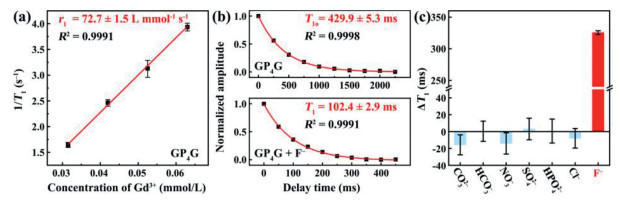
The T1 relaxation times of the GP4G aqueous solutions were measured at 118 µT using a homemade ULF NMR system. The T1 values obtained when the concentration of the Gd3+ is 0.063, 0.053, 0.042, and 0.032 mmol/L are 254.1 ± 4.9, 319.4 ± 16.8, 408.1 ± 10.6, and 607.9 ± 17.9 ms, respectively (Fig. S4 in Supporting information). These data can be plotted in linear form, as shown in Fig. 2a. The longitudinal relaxivity, r1, of the GP4G corresponds to the gradient of the line of best fit which is found to be 72.7 ± 1.5 L mmol‒1 s‒1 (R2 = 0.9991). This is a much larger r1 value compared to those of commercially available Gd3+-based complexes at the same static magnetic field (for example, Gd-EOB-DTPA has an r1 value of 12.3 ± 0.6 L mmol‒1 s‒1) [31]. Such an elevation in relaxivity mainly derives from the localized superacid microenvironment brought by the GQDs [14]. This leads to an enhanced number of exchangeable protons and positively accelerates the proton exchange rate among the protons in coordinated water molecules and free protons (in bulk water or ionized from the GQDs), leading to a high r1 value.
Figure 2
Figure 2.
Magnetic properties of the F‒ detection probe at ULF. (a) Linear fit used to determine the r1 value of the GP4G. (b) Single-exponential fits to find the T1 values of samples. Upper figure: GP4G with Gd3+ (0.042 mmol/L) to determine the relaxation time, T1o, of a blank sample. Lower figure: GP4G with F‒ added (1 mmol/L). (c) Comparison of relaxation time changes (ΔT1) caused by different anions (each at the same concentration of 1 mmol/L). Error bars indicate the standard deviation (SD).
As GP4G has such a high relaxivity, it was employed as a magnetic sensor to detect anions. As a blank control, the T1 value of the GP4G used was first measured, yielding a value of 429.9 ± 5.3 ms with the Gd3+ concentration of 0.042 mmol/L (upper figure in Fig. 2b which shows the best fit to a single exponential function, producing an R2 value of 0.9998). Aqueous F‒ (1 mmol/L) were then mixed with GP4G at room temperature for 12 h and the impact on the relaxivity of the GP4G was determined. The T1 value is found to be strongly reduced to 102.4 ± 2.9 ms (lower figure in Fig. 2b). The change in relaxation time ΔT1 = T1o ‒ T1 is used to quantify the change occurring, where T1o is the relaxation time of the blank sample and T1 is the relaxation time of the sample containing the anion. In this case (using F–), the ΔT1 value is equal to 327.5 ± 2.9 ms which shows that the F‒ undergo a significant interaction with the GP4G.
To evaluate the specificity of the detection method, various other anions CO32−, HCO3−, NO3−, SO42−, HPO42−, and Cl− were detected at the same concentration (1 mmol/L) using the same reaction conditions (room temperature, 12 h). The results (Fig. 2c) clearly indicate that the presence of F– leads to a very large change in relaxation rate (ΔT1 = 327.5 ± 2.9 ms), while the ΔT1 values of the mixtures containing other anions are essentially zero. Thus, the GP4G detection probe has a high specificity towards F–.
The high selectivity and large change in relaxation time of the GP4G suggests that selective coordination between the Gd3+ and F– as well as the localized polarization of water molecules could potentially be involved in the sensing process. Relaxometry experiments and theoretical calculations were therefore carried out to obtain a better understanding of the sensing process.
Ion chromatography was used to determine the concentration of the F‒ present. The concentration of dissociated F‒ is found to be 0.03 µmol/L when 5 mL of aqueous F‒ (0.2 mmol/L) was mixed with 5 mL of the GP4G (the total F‒ concentration in the mixture is 0.1 mmol/L). The obvious decrease in the concentration of dissociated F‒ indicates that the GP4G and F‒ combine together strongly. Indeed, the binding affinity between GP4G and F‒ is 8.3 (logKa value).
Interestingly, the optical properties of GP4G that related to the bandgap or defect/edge states of the GQDs [29, 32] show no obvious changes when F‒ combine with it (Fig. S5 in Supporting information), which means the interaction between GP4G and F‒ has no effect on the GQDs in GP4G. Therefore, the F‒ are probably interacting with the magnetic center in the GP4G (i.e., the Gd3+).
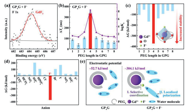
An XPS survey was then carried out to investigate the nature of the interaction between GP4G and F‒. As shown in Figs. S6‒S8 (Supporting information), the peaks in the C 1s, O 1s, and Gd 4d XPS spectra do not change significantly after mixing the GP4G with F‒. On the other hand, the high-resolution XPS F 1s spectrum produced (Fig. 3a) contains a peak located at 684.2 eV, which can be regarded as arising from the coordination of F‒ to the Gd3+ in GP4G (forming GdF3).
Figure 3
Figure 3.
Probing the interaction between Gd3+ and F‒. (a) XPS F 1s spectrum of GP4G + F‒. (b) Two variables highlighting the strength of the interaction between F‒ and GP4G: The different ΔT1 values measured for different GPG samples (histogram) and the logKa values obtained for F– binding to different GPG species (line chart). Error bars indicate SD values. (c) Free energy changes ΔG corresponding to the coordination of an F‒ to different GPG species. The inset depicts the stable hexa-coordinated structure produced with GP4G (the large negative ΔG value indicating high thermodynamic stability). (d) Corresponding ΔG values for the coordination of various anions to GP4G. (e) Schematic illustration of GP4G with and without the presence of F‒. The large negative electrostatic potential highlights the much stronger polarizing power realized after the F‒ becomes coordinated to the GP4G.
It is worth noting that when Gd(NO3)3 (0.1 mmol/L) is used to detect F‒ (0.3 mmol/L, mixed for 12 h at room temperature) it leads to a relatively small change in relaxation time (ΔT1 = ‒157.9 ± 12.1 ms, Fig. S9 in Supporting information). This small change occurs because the binding affinity between the lanthanide complex and F– is fairly weak (logKa = 1.5‒3) [22], despite the fact that lanthanide ions are generally hard Lewis acids [21] and F‒ is a hard Lewis base [2].
Detection experiments were also performed using GPGs with different PEG chain lengths (GPnG, n = 1‒8). The results are shown in Fig. 3b. In each case, the concentration of F‒ was 1 mmol/L and the solutions were mixed at room temperature for 12 h. The ΔT1 values observed with GP1–8G are 87.0 ± 7.6, 38.9 ± 12.4, 104.8 ± 8.6, 333.6 ± 17.3, 105.4 ± 9.7, 84.1 ± 17.4, 62.2 ± 14.4, and 62.9 ± 11.4 ms, respectively. The binding affinities (logKa) between F‒ and GP1–8G species are also plotted in Fig. 3b (1.5, 1.2, 2.5, 8.3, 2.4, 1.6, 1.3, and 1.3, respectively). It is clear that the ΔT1 (333.6 ± 17.3 ms) and logKa (8.3) values obtained for GP4G are much larger than those of the other GPGs. Thus, the F– is much more strongly bound to the Gd3+ when GP4G is used compared to the other GPnG species.
Density functional theory (DFT) calculations were also carried out to further our understanding of the detection mechanism. The changes in Gibbs free energy (ΔG) calculated for the coordination that occurs between an F‒ and the Gd3+ in different GPnG species (n = 1‒8) are shown in Fig. 3c. A lower ΔG value indicates greater thermodynamic stability. As can be seen, the ΔG value calculated for GP4G is much larger in magnitude (‒372.5 kJ/mol) compared to those calculated for the other GPGs (‒50 kJ/mol to ‒170 kJ/mol). This is a clear indication of the stability of the coordination compound formed between GP4G and F‒. That is, the collaborative coordination of the quinquidentate ligand (PEG4) and F‒ forms a stable hexa-coordinated structure with the Gd3+ ion (Fig. 3c). At the same time, the small radius of the F‒ (133 pm) ensures that it can gain close access to the Gd3+ even though there is a large amount of steric hindrance caused by the PEG4 molecule. This allows selective coordination between GP4G and F‒ to be achieved. This can be further highlighted by calculating the ΔG values for other anions coordinating with GP4G (Fig. 3d). As can be seen, only the F– gives a ΔG value that is negative, i.e. GP4G is capable of selective and stable coordination with F‒.
The localized polarization effect experienced by water molecules due to the coordination of the F‒ to the GP4G center can also be demonstrated via DFT calculation. As shown in Fig. 3e, the electrostatic potentials of Gd3+ in GP4G are ‒304.1 and ‒52.7 kJ/mol with and without the presence of F‒, respectively. The large negative electrostatic potential obtained with F– indicates that there is strong charge separation occurring after the F‒ coordinates with the GP4G. This strong charge separation results in the localized polarization of nearby water molecules which makes it easier for the water molecules to become ionized. This means that proton exchange becomes more facile and so the proton exchange rate is enhanced as is the relaxivity, consistent with the experimental results.
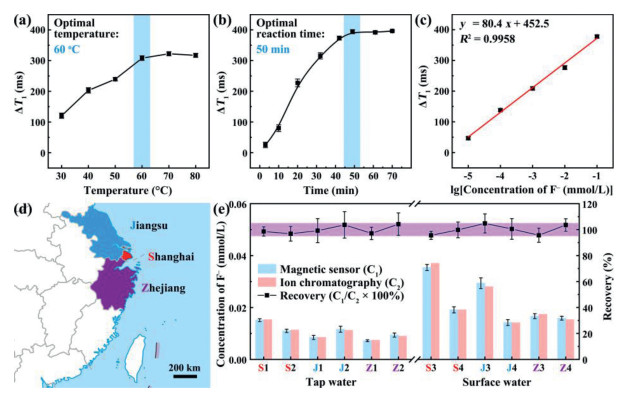
The conditions used when the coordination reaction (between GP4G and F‒) is carried out need to be optimized to ensure the best sensitivity and efficiency is achieved. The efficiency of the reaction between GP4G and F– is mainly governed by the temperature used. A series of experiments were therefore performed using temperatures ranging from 30 ℃ to 80 ℃, giving the results shown in Fig. 4a (the F‒ concentration was fixed at 1 mmol/L and the coordination process was allowed to proceed for 30 min in each case). The ΔT1 value of the coordination product was then measured. Clearly, the ΔT1 values increase as the reaction temperature is increased. When a temperature of 60 ℃ was used, the ΔT1 value was found to be 308.2 ± 7.6 ms. Further increasing the reaction temperature only led to a slight increase in ΔT1 value (by ~15.0 ms). Therefore, the optimal reaction temperature for detecting F– using GP4G is taken to be 60 ℃.
Figure 4
Figure 4.
Optimization of: (a) reaction temperature, and (b) reaction time for the coordination reaction between F– and GP4G. The F– concentration is 1 mol/L in each case. (c) The linear relationship between ΔT1 and logarithm of the F– concentration. (d) The area from which water was collected. This image is a modified version of a map provided by the map service administrated by the Ministry of Natural Resources of the People's Republic of China. (e) Comparison of the F– concentrations measured using the magnetic sensor (C1) and ion chromatography (C2). The upper trace shows the recovery values (C1/C2 × 100%) which help illustrate the accuracy of the magnetic sensor. The band underneath the trace represents the recovery range 95%–105%. Error bars indicate SD values (For interpretation of the references to color in this figure, the reader is referred to the web version of this article.).
The optimal reaction time can be determined by monitoring ΔT1 every 10 min as the reaction proceeds (at 60 ℃). Fig. 4b shows the results obtained. The ΔT1 value clearly increases as the reaction between GP4G and F– proceeds and it eventually levels off and approaches a constant value as the reaction approaches completion. The optimal reaction time is taken to be 50 min, whereupon ΔT1 reaches 394.2 ± 6.5 ms (after this time, there is no significant change in the recorded relaxation time).
The magnetic stability of GP4G was also investigated by measuring its T1 relaxation time over an extended period of time (3 months, Fig. S10 in Supporting information). The results proved that the probe can be stored for a long period of time without any significant changes in magnetic properties.
The relaxation times of F– solutions with a variety of different known concentrations were measured using the optimal reaction conditions (60 ℃, 50 min). A wide range of concentrations from 0.1 nmol/L to 1 mmol/L were used, giving the results shown in Fig. S11 (Supporting information). Clearly, ΔT1 increases with increased F– concentration. According to Fig. S11 (Supporting information), the limit of detection (LOD) of the detection method is 10 nmol/L (corresponding to the F– concentration that produces a ΔT1 value just larger than that of a blank sample plus 3 SDs, here, the ΔT1 value of a blank sample is 0 ms and the SD is 6.3 ms). This LOD is about 3 orders of magnitude lower than that specified in the World Health Organization guidelines (79 µmol/L) [33]. Fig. S12 (Supporting information) compares our result with the LODs of other F– detection methods and reveals that the magnetic sensor we propose thus has excellent sensitivity and should be capable of detecting very low levels of F– in real samples.
Moreover, the linearity of the relationship between ΔT1 and the logarithm of the F– concentration is excellent over the range from 10 nmol/L to 0.1 mmol/L (Fig. 4c, where R2 = 0.9958). This means that Fig. 4c can be used as a calibration curve that can be used to detect F– quantitatively over a wide range of concentrations.
Fluoride is known to play a major role in preventing dental caries [34] and it is also used to treat osteoporosis [35]. It is easily absorbed by the body but is excreted slowly. As a result, overexposure to fluoride can increase the risk of acute gastric [2], dental fluorosis [33], skeletal fluorosis [36], and kidney problems [37]. Given that domestic drinking water generally contains F‒, tap and surface water are the two most common water sources we are exposed to. Therefore, we collected water samples (tap and surface) from the Yangtze River Delta region of China, i.e. Shanghai City, Jiangsu Province, and Zhejiang Province (Fig. 4d) and determined the concentration of F‒ in them using the newly developed magnetic sensor.
The labels S1‒2 (S3‒4), J1‒2 (J3‒4), and Z1‒2 (Z3‒4) are used to denote samples of tap (surface) water collected from Shanghai City, Jiangsu Province, and Zhejiang Province, respectively. The concentrations of the F– in the samples were then determined using the magnetic sensor and the calibration curve shown in Fig. 4c. The resulting concentrations are highly consistent with those obtained using ion chromatography (Fig. 4e, Tables S1 and S2 in Supporting information). In Fig. 4e, the histogram shows the concentrations as determined using the magnetic sensor (C1 in light blue) and ion chromatography (C2 in light red). No significant differences were observed between the C1 and C2 values obtained for samples with the same sample label. Fig. 4e also shows a plot of the 'recovery' of the magnetic sensor which is defined as the quotient C1/C2. As can be seen, the recovery stays very close to 1 which indicates that the magnetic sensor has a high reliability.
To conclude, we have demonstrated that it is possible to achieve controllable and selective coordination to Gd3+ by adjusting the length of the PEG chain incorporated into the magnetic GQDs. Strong binding occurs between the magnetic GQDs and F‒ (logKa = 8.3) when the PEG used is tetraethylene glycol. The combination, in fact, is more stable than those between other lanthanide complexes and F‒. When an F‒ is selectively and stably coordinated to the Gd3+, the bulk water around the GP4G nanoparticle is strongly polarized and more easily ionized. This provides more exchangeable protons and thus increases the proton exchange rate. These changes in microenvironment lead to a decrease in the T1 observed via ULF NMR relaxometry. The change in T1 value is intimately connected with the concentration of the F– in the original solution which means the technique can be used for quantitative analysis. The LOD of the F‒ detection technique was found to be 10 nmol/L. A series of experiments involving domestic water samples were also carried out to illustrate the accuracy of the detection method. This work should inspire the formulation of other similar magnetic probes for anion sensing. It should also be of great interest to researchers designing high-relaxivity contrast agents for use in magnetic resonance imaging.
Declaration of competing interest
The authors declare no competing financial interest.
Acknowledgments
The authors would like to thank Dr. Gang Wang (Ningbo University) for collecting the water samples used in this work. This work was financially supported by the National Natural Science Foundation of China (Nos. 11874378, 11804353, and 11774368), and the Science and Technology Commission of Shanghai Municipality (Nos. 19511107100, 19511107400).
Supplementary materials
Supplementary material associated with this article can be found, in the online version, at doi:10.1016/j.cclet.2021.05.014.
[1]
S.S. Razi, R.C. Gupta, R. Ali, et al., Sens. Actuators B Chem.236 (2016) 520–528 doi: 10.1016/j.snb.2016.06.016
[2]
Y. Zhou, J.F. Zhang, J. Yoon, Chem. Rev. 114 (2014) 5511–5571 doi: 10.1021/cr400352m
[3]
A. Kumar, M. Bhatt, G. Vyas, S. Bhatt, P. Paul, ACS Appl. Mater. Interfaces9 (2017) 17360–17369
Z.P. Liang, P.C. Lauterbur, Principles of Magnetic Resonance Imaging: a Signal Processing Perspective, SPIE Optical Engineering Press, Bellingham, 2000, pp. 2–4
[8]
H.J. Chung, C.M. Castro, H. Im, H. Lee, R. Weissleder, Nat. Nanotechnol. 8 (2013) 369–375 doi: 10.1038/nnano.2013.70
[9]
W.J. Lu, Y.P. Chen, Z. Liu, et al., ACS Nano10 (2016) 6685–6692 doi: 10.1021/acsnano.6b01903
[10]
H. Lee, T.J. Yoon, R. Weissleder, Angew. Chem., Int. Ed. 48 (2009) 5657–5660 doi: 10.1002/anie.200901791
[11]
Z.C. Xu, C. Liu, S.J. Zhao, S. Chen, Y.C. Zhao, Chem. Rev. 119 (2019) 195–230 doi: 10.1021/acs.chemrev.8b00202
[12]
K. Kattel, J.Y. Park, W.L. Xu, et al., ACS Appl. Mater. Interfaces3 (2011) 3325–3334 doi: 10.1021/am200437r
[13]
J. Wahsner, E.M. Gale, A. Rodriguez-Rodriguez, P. Caravan, Chem. Rev. 119 (2019) 957–1057 doi: 10.1021/acs.chemrev.8b00363
World Health Organization, Guidelines For Drinking-Water Quality, in: Guidelines For Drinking-Water Quality, 4th Ed., World Health Organization, 2011, pp. 1–564.
[34]
K.L. Kirk, Biochemistry of the Elemental Halogens and Inorganic Halides, Plenum Press, New York, 1991
Y. Michigami, Y. Kuroda, K. Ueda, Y. Yamamoto, Anal. Chim. Acta274 (1993) 299–302 doi: 10.1016/0003-2670(93)80479-5
Figure 1
(a) TEM image of GP4G, (b) size distribution histogram (and the corresponding fit to a Gaussian distribution function), and (c) a HR-TEM image of GP4G in which the regular hexagons (white lines) outline the graphene structure. (d) Topographical AFM image of GP4G nanoparticles on a 300 nm SiO2/Si substrate. Inset: height profiles along the lines indicated. The final images are XPS spectra of the GP4G nanoparticles corresponding to (e) C 1s, and (f) O 1s signals.
Figure 2
Magnetic properties of the F‒ detection probe at ULF. (a) Linear fit used to determine the r1 value of the GP4G. (b) Single-exponential fits to find the T1 values of samples. Upper figure: GP4G with Gd3+ (0.042 mmol/L) to determine the relaxation time, T1o, of a blank sample. Lower figure: GP4G with F‒ added (1 mmol/L). (c) Comparison of relaxation time changes (ΔT1) caused by different anions (each at the same concentration of 1 mmol/L). Error bars indicate the standard deviation (SD).
Figure 3
Probing the interaction between Gd3+ and F‒. (a) XPS F 1s spectrum of GP4G + F‒. (b) Two variables highlighting the strength of the interaction between F‒ and GP4G: The different ΔT1 values measured for different GPG samples (histogram) and the logKa values obtained for F– binding to different GPG species (line chart). Error bars indicate SD values. (c) Free energy changes ΔG corresponding to the coordination of an F‒ to different GPG species. The inset depicts the stable hexa-coordinated structure produced with GP4G (the large negative ΔG value indicating high thermodynamic stability). (d) Corresponding ΔG values for the coordination of various anions to GP4G. (e) Schematic illustration of GP4G with and without the presence of F‒. The large negative electrostatic potential highlights the much stronger polarizing power realized after the F‒ becomes coordinated to the GP4G.
Figure 4
Optimization of: (a) reaction temperature, and (b) reaction time for the coordination reaction between F– and GP4G. The F– concentration is 1 mol/L in each case. (c) The linear relationship between ΔT1 and logarithm of the F– concentration. (d) The area from which water was collected. This image is a modified version of a map provided by the map service administrated by the Ministry of Natural Resources of the People's Republic of China. (e) Comparison of the F– concentrations measured using the magnetic sensor (C1) and ion chromatography (C2). The upper trace shows the recovery values (C1/C2 × 100%) which help illustrate the accuracy of the magnetic sensor. The band underneath the trace represents the recovery range 95%–105%. Error bars indicate SD values (For interpretation of the references to color in this figure, the reader is referred to the web version of this article.).

 DownLoad:

 下载:
下载: