Citation:
Haicheng Lv, Jundi Wang, Zhongming Shu, Gang Qian, Xuezhi Duan, Zhirong Yang, Xinggui Zhou, Jing Zhang. Residence time distribution and heat/mass transfer performance of a millimeter scale butterfly-shaped reactor[J]. Chinese Chemical Letters,
2023, 34(4): 107710.
doi:
10.1016/j.cclet.2022.07.053
Residence time distribution and heat/mass transfer performance of a millimeter scale butterfly-shaped reactor
English
Residence time distribution and heat/mass transfer performance of a millimeter scale butterfly-shaped reactor
Received Date:
25 May 2022 Accepted Date:
26 July 2022 Revised Date:
22 July 2022 Available Online:
15 April 2023
Abstract:
A millimeter scale butterfly-shaped reactor was proposed based on sizing-up strategy and fabricated via femtosecond laser engraving. An improvement of mixing performance and residence time distribution was realized by means of contraction and expansion of the reaction channel. The liquid holdup was greatly increased through connection of multiple mixing units. Structure optimization of the reactor was carried out by computational fluid dynamics simulation, from which the effect of reactor internals on mixing and the influence of parallel branching structure on heat transfer were discussed. The UV–vis absorption spectroscopy was used to determine the residence time distribution in the reactor, and characteristic parameters such as skewness and dimensionless variance were obtained. Further, a chained stagnant flow model was proposed to precisely describe the trailing phenomenon caused by fluid stagnation and laminar flow in small scale reactors, which enables a better fit for the experimental results of the asymmetric residence time distribution. In addition, the heat transfer performance of the reactor was investigated, and the overall heat transfer coefficient was 110–600 W m-2 K-1 in the flow rate range of 10–40 mL/min.
Microfluidic technology is an important approach to realize process intensification and safe operation. It has unique advantages over traditional reactors due to precise control and efficient heat/mass transfer. Nevertheless, the flow in the microchannel is mainly laminar flow with wide residence time distribution (RTD) and large back mixing, which may adversely affect the conversion and selectivity control of chemical reactions. Meanwhile, higher liquid holdup of microreactor is often desired for many reactions and industrial demands.
To increase the liquid holdup, the scaling up strategies of microreactors are mainly divided into two categories, numbering up and sizing up [1]. Numbering up is simple and convenient, but often requires relatively high investment in equipment. Also, uniform fluid distribution within each channel/unit needs to be addressed during numbering up [2, 3]. With widespread industrial applications of reactors with channel sizes in the range of sub-millimeter to millimeter [4-8], many studies began to explore sizing up strategies [9-11]. The sizing up strategy is able to maintain the reactor channel number and increase tolerance for solids-containing reactions [12], but may compromise its heat/mass transfer efficiency. Therefore, a proper combination of intensification strategies is required to achieve good mixing within the scaled-up reactor. The strategies of mixing intensification usually include "active mixing" and "passive mixing". The "active mixing" often requires complex structures and faces difficulty in assembly, so the development of which remains in research lab. In contrast, the "passive mixing" usually adopts certain measures to divide, recombine, shear, stretch and fold the fluid to reduce the thickness of the liquid layer and has many practical applications [13]. Therefore, many passive mixing reactors were designed as serpentine [14], zigzag [15], irregular structures [16, 17] or channels with internal obstacles [18, 19], which can generate local disturbances to enhance the mixing process. In addition, the heat transfer efficiency of reactor is also significant for its industrial application, where the precise control of temperature can be beneficial to selectivity. In this regard, the following three strategies are usually used: choosing materials with high thermal conductivity (e.g., Hastelloy [20], silicon carbide [21]), reducing wall thickness, and increasing heat transfer area. For reactors made of glass, due to the limitations of its thermal conductivity and hardness, the heat transfer performance can often only be improved by reasonable structural design, such as parallel branching structure [22] to improve the uniformity of the heat transfer fluid. Such structural design and optimization are usually carried out using computational fluid dynamics (CFD) by simulating the flow over different structures.
A narrow RTD is important to precisely control the conversion and yield of chemical reactions [23, 24]. However, the predominance of laminar flow in the microchannels usually results in a relatively wide RTD of the tracer material at the outlet [25]. Therefore, many studies have used the RTD as an important criterion for the performance of small scale reactors [26]. The small size of such reactors makes the traditional method via conductivity measurement being ineffective. As a result, new detection methods and devices are required, such as fluorescence microscopy [27] and continuous UV–vis absorption spectroscopy [28]. A further combination of experimental results and flow models can be used to predict the performance of non-ideal flow reactors [29]. Ideal flow models usually consist of plug flow model and complete mixing model. However, in actual reactors, the flow velocity distribution is often not uniform. Also, the presence of reactor internals can cause reverse flow or stagnation zones, resulting in flow deviating from the ideal flow state. Common non-ideal flow models include laminar flow model, axial diffusion model and tank-in-series model. The laminar flow model is suitable for laminar or viscous flows in short channels [30], while the axial diffusion model and the tank-in-series model are suitable for flows close to plug flow or complete mixing flow [31, 32]. However, for the flow in small scale channels, the outlet concentration distribution of the tracer material is often subject to a combination of (laminar) flow and diffusion. So the above models are often biased in terms of skewness and peak value [33], making them difficult to describe the actual flow process.
Enhancement of processing capacity is vital to the development of microreactor technology and its industrial application. In this regard, reactors of millimeter scale may have both decent liquid holdup and heat/mass transfer efficiency. In the current study, a millimeter scale butterfly-shaped glass reactor was designed via CFD simulation and fabricated via femtosecond laser engraving. An improvement of mixing performance and residence time distribution was realized by means of contraction and expansion of the reaction channel. The liquid holdup was greatly increased through connection of multiple mixing units. The RTD and heat transfer performance of the reactor were investigated, and a flow model was established to accurately describe the flow at small-length scales with a smaller fitting deviation than the existing flow model.
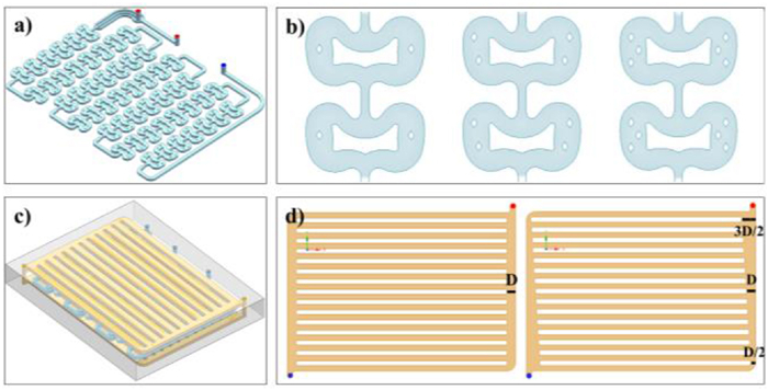
Firstly, the structures of different reactors were compared by CFD simulations. Guided by the principle of split-and-recombine configuration, a butterfly-shaped reactor was proposed, the design concept of which was provided in Fig. S1 (Supporting information). The butterfly-shaped reactor consists of three parts: the reaction layer, the heat exchange layer and the glass matrix. As shown in Fig. 1a, the reaction channel consists of multiple mixing units in series, and the size of each mixing unit was 15 mm × 8.8 mm × 1.2 mm with an internal volume of 112 µL. A butterfly-shaped obstacle was set up in the middle of each mixing unit, and pairs of internals (rhombus microcolumns or circle microclumns) were arranged on both sides (the detialed information are shown in Figs. S2-S4 in Supporting information). The geometric model with different pairs of internals were considered as shown in Fig. 1b. As shown in Fig. 1d, the heat exchange channels adopt parallel branching structure, and two types of arrangements, equal width and gradual width, were considered respectively. The simulation adopts 3D model, and the configuration of the reactor is shown in Fig. 1c, where the middle part is the butterfly-shaped reaction channel and the upper/lower parts are the heat exchange layers. Details of the simulation are shown in Supporting information.
Figure 1
Figure 1.
Geometric model of the reactor: (a) The overall reaction channel; (b) The mixing unit with different internals; (c) The whole reactor with reaction and heat exchange channels; (d) The heat exchange channel with different structures.
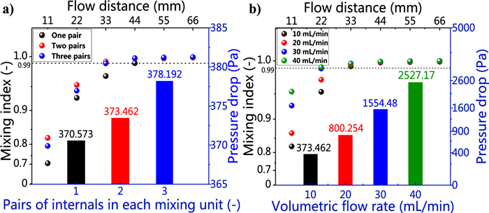
The reaction channel used water and ethanol as fluids to simulate the homogeneous mixing process, and the mixing index M was used to evaluate the degree of mixing [34], the closer the M value is to 1, the more complete the mixing is, and vice versa. Since the mixing process is rapid and the complete mixing can be reached within a short distance, the simulation results were analyzed only for the first six mixing units. As shown in Fig. 2, a cross-section was taken at the outlet of each mixing unit, and enough data points were selected on each cross-section, so the mixing index of each cross-section can be calculated (the calculation equation is shown in Supporting information). As shown in Fig. 3a, the pressure drop increases gradually with the increasing number of internals, while the mixing index for homogeneous mixing increases first and then decreases. This is due to the local turbulence (velocity gradient) is enhanced as the number of internals increases, but at the same time, the mixing time in a single unit is shortened, thereby reducing the degree of mixing at the outlet. Therefore, the mixing process needs to consider the effects of both aspects. In the current study, the structure with two pairs of internals is desired. Further, the mixing index and pressure drop at different flow rates were compared and the results are shown in Fig. 3b, where both the mixing index and pressure drop increased with increasing flow rate. Using M > 99% as the standard for complete mixing, the mixing time in the flow rate range of 10–40 mL/min was about 0.35–2.1 s. The velocity fields and streamlines at different total flow rates are shown in Fig. S5 (Supporting information).
Figure 2
Figure 2.
Schematic diagram of the cross-sections for mixing index analysis in Fig. 3.
Figure 3.
Mixing index and pressure drop of the reactor (based on six mixing units): (a) Effect of the number of internals in each mixing unit; (b) Effect of flow rates.
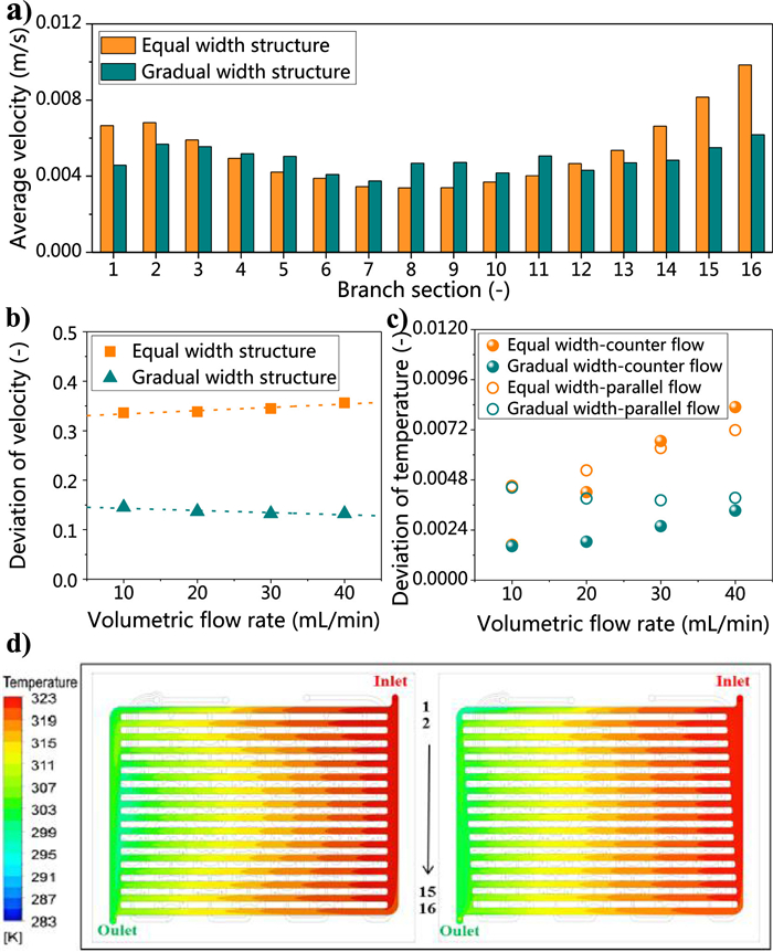
The heat transfer channel used hot and cold water as fluid to simulate the heat transfer process. The flow velocity V of each branch pipe and the standard deviation D of the velocity were used to quantitatively evaluate the uniformity of the fluid distribution under different conditions and structures (calculation equations are shown in Supporting information). The average flow velocity of each branch pipe for the two heat transfer channel structures at the same volumetric flow rate is shown in Fig. 4a, the flow velocity of the equal width structure ranges from 0.0034 m/s to 0.0099 m/s, and the flow velocity of each branch near the inlet and outlet (1–2, 15–16) is larger, while the flow velocity of each branch near the middle area is smaller. In contrast, the uniformity of flow velocity distribution for the heat transfer with gradual width structure is significantly improved, where the flow velocity ranges from 0.0038 m/s to 0.0062 m/s with decreased flow velocity of branches near the inlet and outlet and increased flow velocity of branches near the middle region. The standard deviations of flow velocities for the two heat transfer channel structures are shown in Fig. 4b, at the same flow rate, the velocity standard deviation of heat transfer channel with gradual width structure is much smaller than the one with equal width structure. Fig. 4d shows the temperature distribution within different heat transfer channel in the reaction channel. The comparison shows that the temperature distribution within each branch of the gradual width structure is more uniform than that of the equal width structure. The results of the standard deviations of the temperature distributions within the two heat transfer channel structures at different flow rates and heat transfer modes are shown in Fig. 4c. The results show that the temperature distribution deviation of the gradual width structure is smaller than that of the equal width structure under the same flow rate or heat transfer mode, and the difference between them increases gradually with the increasing flow rate. Thus, the gradual width structure leads to better uniformity in temperature distribution as compared to the equal width structure.
Figure 4
Figure 4.
Velocity and temperature distribution within heat transfer channels of different structures: (a) Average velocity of each branch at a flow rate of 40 mL/min; (b) Standard deviation of velocity at different flow rates; (c) Standard deviation of temperature at different flow rates (hot fluid flow rate is fixed at 40 mL/min); (d) Schematic diagram of temperature distribution (hot fluid flow rate is 40 mL/min, cold fluid flow rate is 20 mL/min).
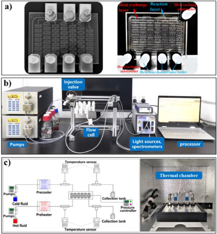
Then, the fabrication of the reactor was performed via femtosecond laser engraving technology, from which two sets of reactors were processed: the one with heat exchange layer and the one without heat exchange layer (Fig. 5a and Table S1 in Supporting information). The experimental setup for the RTD is shown in Fig. 5b), which consists a manual sample injection valve with a 10 µL sample loop (Xinlimei Technology Co., Ltd.), a flow cell (AVENTES Flow-cell-Z-1.5), a light source (AVENTES AvaLight-DHS), a micro-spectrometer (AVENTES AvaSpec-ULS2048XL-EVO) and a processor. The residence time distribution was determined by the stimulus-response method, using deionized water as the flow medium and sodium fluorescein (2.5 g/L) as the tracer. Shortest possible PTFE tubes (0.5 mm ID) were used to connect the reactor to the sample injection valve and the flow cell. The experimental data were the average values from triplicate runs. The scheme for the overall heat transfer coefficient measurement is shown in Fig. 5c. Firstly, the hot and cold fluids were pre-heated and pre-cooled, then fed into the inlets of the reaction channel and the heat exchange channel, respectively, and indirectly heat exchange through the solid wall, and finally flowed out through the outlets of the reaction channel and the heat exchange channel (the experimental setup diagram is shown in Fig. S6 (Supporting information)). A temperature sensor was placed at both the inlet and outlet of the reactor to measure the time-on-stream temperature of the fluid. The reactor and temperature sensor were placed in the thermal chamber, the structure of which is shown in Fig. 5c.
Figure 5
Figure 5.
Experimental equipment: (a) Photos of the reactor (left: without heat transfer layer; right: with heat transfer layer); (b) Photo for RTD measurement; (c) Schematic diagram of the heat transfer experiment and photo of the thermal chamber.
The maximum absorption wavelength of the fluorescent substance (tracer) was used for collection of UV spectrogram. As shown in Fig. 6a, a scan was performed in the wavelength range of 180 nm-1100 nm, and the results showed that the maximum absorption wavelength of the tracer was 483.5 nm. The reproducibility of the experiments was evaluated in Fig. 6b, and the relative errors of the absorbance-time curves (run 1–3) of the three parallel experiments were within 5% at a volume flow rate of 30 mL/min. Fig. 6c shows the absorbance response curves at flow rates of 10–40 mL/min. As the flow rate increased, the response time became shorter and the peak height of the response curve became higher. The dimensionless RTD curves are shown in Fig. 6d, with the increase of the flow rate, the convection rate is enhanced and the effect of the axial diffusion rate is weakened, resulting in a narrower RTD density function curve and a shorter trailing length of the curve. The numerical characteristics of the mean residence time, skewness and dimensionless variance of RTD at different flow rates are presented in Table 1. From the dimensionless variance results, an increase of volumetric flow rate intensified the convective flow and makes the breakthrough time of the tracer more concentrated. From the skewness results, the RTD curves are asymmetric left skewed curves at all flow rates, which are mainly caused by two reasons. Firstly, the laminar flow in the reaction channel leads to a radial concentration distribution, so that the tracer at the center of the channel reaches the reactor outlet first while the tracer near the wall is detained, resulting in a long trailing. Secondly, the internal structure of the butterfly-shaped mixing unit causes fluid stagnation in some regions. Although most tracer bypasses these regions and reaches the reactor outlet, some tracer may take longer to reach the outlet once entering these stagnant regions, making a wider RTD curve.
Figure 6
Figure 6.
Experimental results of RTD in the reactor with 51 mixing units. (a) Full-band spectrum of the tracer; (b) Producibility of the absorbance response curve at a flow rate of 30 mL/min; (c) Absorbance response curves; (d) Dimensionless RTD curve.
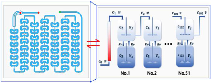
The current study proposed a chained stagnation flow model to describe the RTD of small scale reactors given the effects of laminar flow and stagnation zone on the RTD, and a comparison with common flow models was made. The principle of the model is shown in Fig. 7, where each mixing unit is considered as a combination of two parts: "flow zone (light blue)" and "stagnation zone (dark blue)", and the concentration distribution at its outlet is used as the inlet concentration of the next mixing unit. As a result, 51 such combinations can be used to predict the concentration distribution at the outlet of the last mixing unit. The model adopts two parameters, volume ratio p (ratio of "stagnation zone" to "flow zone") and recycle ratio R (ratio of "fluid exchange rate" to "total flow rate"), to describe the internal flow characteristics for each mixing unit. At the same time, the pipes other than the mixing unit (inlet, outlet and each connecting pipe) are considered as laminar flow and are equated by a portion of inlet pipe to characterize the effect of laminar flow on the whole flow process. The details of the solution of differential equations of this model are shown in the Supporting information.
Figure 7
Figure 7.
Schematic diagram of the reactor and flow model.
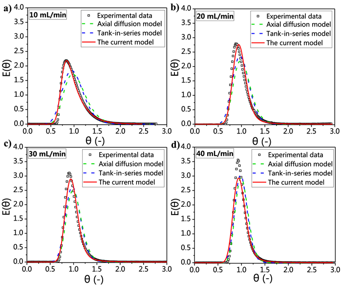
According to the experimental results and the flow model equation, the parameter of each model can be obtained in Table 2. The fitting results of each flow model at different flow rates are shown in Fig. 8. Compared with other flow models, the current flow model is more accurate in describing the laminar flow behavior in small scale reaction channels. Especially at low flow rates, the RTD curves obtained by the current model are very close to the experimental results. In contrast, the curves obtained by the axial diffusion model and the tank-in-series model were highly symmetric under the current flow range, which differs significantly from the experimental results. This is because that the above models are based on the ideal flow state (plug flow or complete mixing flow), while the existence of boundary layer in the actual flow process will make the RTD curve has a certain degree of skew. By introducing two factors, the volume ratio and recycle ratio, the current model can precisely describe the trailing phenomenon caused by fluid stagnation, resulting in a better fitting for the experimental results of asymmetric RTD. In addition, since the current model is based on the number of actual mixing units (m = 51), and the volume ratio and recycle ratios are fixed at the same flow rate, it provides better extrapolation than the conventional tank-in-series model.
Figure 8.
Comparison of dimensionless RTD curves from different flow models and experimental data at various flow rates: (a) 10 mL/min; (b) 20 mL/min; (c) 30 mL/min; (d) 40 mL/min.
The parameters of the current flow model are shown in Table 3. Under the same volume ratio, the time for the particles to return to the flow body from the stagnation zone is shortened with increasing recycle ratio, resulting in a decrease of the dimensionless variance, which illustrates the intensification of the mass transfer by the fluid flow. When the recycle ratio is very small, only one CSTR (stagnation zone) is at play in the two parts (stagnation zone and flow zone); whereas when the recycle ratio is large, the two parts behave together as one CSTR, where the volume ratio has little effect on the dimensionless variance. Therefore, a fixed value of the volume ratio is used in this study.
Table 3
Table 3.
Parameters of the current flow model, chained stagnation flow model.
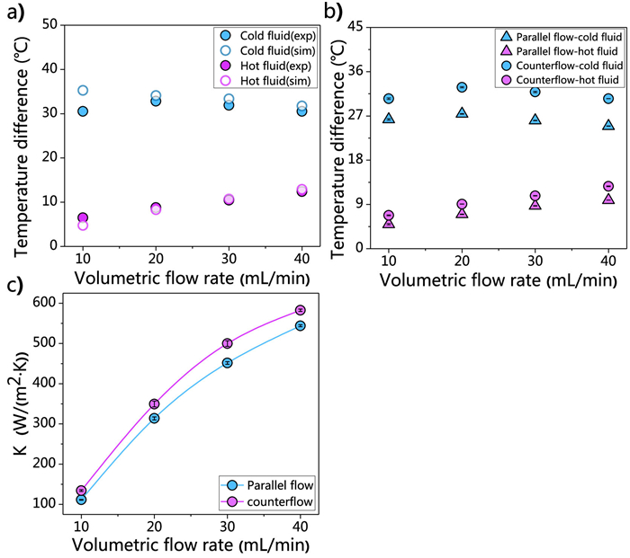
For the heat exchange experiments, since the inlet temperature of the hot and cold fluid will deviate from the set temperature due to the heat exchange between the fluid medium and the environment in the pipeline before entering the reactor. Therefore, to evaluate the heat exchange effect under different flow rates more accurately, the temperature difference between the inlet and outlet of the fluid were taken as the basis for evaluation. A comparison between simulation and experimental results is shown in Fig. 9a, where the results agree well with each other at flow rates higher than 10 mL/min. A small deviation was observed at the flow rate of 10 mL/min, possibly due to the non-negligible heat dissipation of the cold fluid at the low flow rate leading to a lower outlet temperature than the theoretical result. As shown in Fig. 9b. When the cold fluid flow rate increases, more heat was utilized for heating the cold fluid, leading to a larger temperature difference between the inlet and outlet of the hot fluid in the heat transfer channel, while the opposite was true for the cold fluid in the reaction channel. Since the environmental temperature is significantly lower than the inlet temperature of the hot fluid during the experiment, the heat loss of the hot fluid is much greater than that of the cold fluid. Therefore, the temperature difference of the cold fluid was used as the basis to calculate the overall heat transfer coefficient to improve the accuracy. As shown in Fig. 9c, the overall heat transfer coefficient is 110–600 W m-2 K-1 in the flow rate range of 10–40 mL/min. Moreover, the overall heat transfer coefficient of the counterflow heat transfer is slightly higher than that of the parallel flow heat transfer at the same flow rate. As shown in Table 4, the heat transfer performance is comparable to the Corning Advanced Flow Reactor [35].
Figure 9
Figure 9.
Results of the heat transfer experiment: (a) Comparison of inlet and outlet temperature difference between simulation and experimental results (counterflow); (b) Temperature difference between hot and cold fluid inlet and outlet; (c) Overall heat transfer coefficient.
In conclusion, the design and fabrication of a millimeter scale reactor was carried out using computational fluid dynamics and femtosecond laser engraving, the RTD and heat transfer of which were investigated experimentally. The results show that by arranging two pairs of rhombus internals alternately in each butterfly-shaped mixing unit, the degree of radial mixing can be improved while maintaining a low pressure drop. For the heat exchange channel, parallel branches with gradual width structure lead to more uniform flow distribution and thus more uniform temperature distribution, resulting in overall heat transfer coefficients up to 600 W m-2 K-1. The narrowness and symmetry of the RTD were significantly improved by series connection of multiple butterfly-shaped mixing units. Further, a chained stagnant flow model was proposed to precisely describe the trailing phenomenon caused by fluid stagnation and laminar flow in small scale reactors, enabling a better fit for the experimental results of asymmetric RTD, as compared to the existing flow models.
Declaration of competing interest
The authors declare that they have no known competing financial interests or personal relationships that could have appeared to influence the work reported in this paper.
Acknowledgments
This research was funded by the National Natural Science Foundation of China (Nos. 21991103, 21991104, 22008074, 22008072); Natural Science Foundation of Shanghai (No. 20ZR1415700), China Postdoctoral Science Foundation (Nos. 2020M671025, 2019TQ0093). The authors thank Prof. Ya Cheng and Dr. Miao Wu from East China Normal University for the fabrication of reactor via femtosecond laser engraving.
Supplementary materials
Supplementary material associated with this article can be found, in the online version, at doi:10.1016/j.cclet.2022.07.053.
[1]
Z.Y. Dong, Z.H. Wen, F. Zhao, S. Kuhn, T. Noël, Chem. Eng. Sci. 10 (2021) 100097.
L.H. Lu, K.S. Ryu, C. Liu, J. Microelectromech. Syst. 11 (2002) 462–469. doi: 10.1109/JMEMS.2002.802899
[35]
M.S. Chivilikhin, V. Soboleva, L. Kuandykov, P. Woehl, E.D. Lavric, Chem. Eng. Trans. 21 (2010) 1099–1104. doi: 10.3303/CET1021184
Figure 1
Geometric model of the reactor: (a) The overall reaction channel; (b) The mixing unit with different internals; (c) The whole reactor with reaction and heat exchange channels; (d) The heat exchange channel with different structures.
Figure 3
Mixing index and pressure drop of the reactor (based on six mixing units): (a) Effect of the number of internals in each mixing unit; (b) Effect of flow rates.
Figure 4
Velocity and temperature distribution within heat transfer channels of different structures: (a) Average velocity of each branch at a flow rate of 40 mL/min; (b) Standard deviation of velocity at different flow rates; (c) Standard deviation of temperature at different flow rates (hot fluid flow rate is fixed at 40 mL/min); (d) Schematic diagram of temperature distribution (hot fluid flow rate is 40 mL/min, cold fluid flow rate is 20 mL/min).
Figure 5
Experimental equipment: (a) Photos of the reactor (left: without heat transfer layer; right: with heat transfer layer); (b) Photo for RTD measurement; (c) Schematic diagram of the heat transfer experiment and photo of the thermal chamber.
Figure 6
Experimental results of RTD in the reactor with 51 mixing units. (a) Full-band spectrum of the tracer; (b) Producibility of the absorbance response curve at a flow rate of 30 mL/min; (c) Absorbance response curves; (d) Dimensionless RTD curve.
Figure 8
Comparison of dimensionless RTD curves from different flow models and experimental data at various flow rates: (a) 10 mL/min; (b) 20 mL/min; (c) 30 mL/min; (d) 40 mL/min.
Figure 9
Results of the heat transfer experiment: (a) Comparison of inlet and outlet temperature difference between simulation and experimental results (counterflow); (b) Temperature difference between hot and cold fluid inlet and outlet; (c) Overall heat transfer coefficient.

 DownLoad:


 下载:
下载: