High Magnetic Field Laboratory, Hefei Institutes of Physical Science, Chinese Academy of Sciences, Hefei 230031, China
b.
The First Affiliated Hospital of USTC, Division of Life Sciences and Medicine, and Center for BioAnalytical Chemistry, University of Science and Technology of China, Hefei 230026, China
Received Date:
23 November 2021 Accepted Date:
24 April 2022 Revised Date:
22 April 2022 Available Online:
15 January 2023
Abstract:
The fluorescence lifetime of nicotinamide adenine dinucleotide (NADH), a key endogenous coenzyme and metabolic biomarker, can reflect the metabolic state of cells. To implement metabolic imaging of brain tissue at high resolution, we assembled a two-photon fluorescence lifetime imaging microscopy (FLIM) platform and verified the feasibility and stability of NADH-based two-photon FLIM in paraformaldehyde-fixed mouse cerebral slices. Furthermore, NADH based metabolic state oscillation was observed in cerebral nuclei suprachiasmatic nucleus (SCN). The free NADH fraction displayed a relatively lower level in the daytime than at the onset of night, and an ultradian oscillation at night was observed. Through the combination of high-resolution imaging and immunostaining data, the metabolic tendency of different cell types was detected after the first two hours of the day and at night. Thus, two-photon FLIM analysis of NADH in paraformaldehyde-fixed cerebral slices provides a high-resolution and label-free method to explore the metabolic state of deep brain regions.
The metabolic state is the sum of the biochemical processes that produce or consume energy in living cells. An abnormal metabolism is often associated with many human diseases, such as cancer [1]. Nicotinamide adenine dinucleotide (NADH) is the key reduced-state coenzyme involved in energy metabolism. Intracellular NADH can exist in either a free state or a protein-bound state [2, 3]. Cell hypoxia causes an increase in glycolysis level and a concurrent increase in the fraction of free NADH. When cells require large amounts of biosynthesis, as is true of stem cells, proliferating cells and cancer cells, elevated glycolysis level occurs within cells to meet the demands of large amounts of carbon and rapid ATP production, despite being in an aerobic environment. Concurrently, the fraction of free NADH increases [4-7]. This means that free NADH exists in the cytoplasmic matrix with vigorous glycolysis, while protein-bound NADH is more strongly associated with mitochondria with TCA and oxidative phosphorylation. Therefore, the relative levels of NADH can shed light on metabolic alterations in cells or tissues.
To assess the metabolic state of cells or tissues, numerous methods have been developed to track cellular metabolic alterations [8-10]. Brain tissue is known to be highly sensitive to the oxygen level of the environment [11] and brain metabolism imaging is important to understand complex brain function and pathological alterations [12]. Currently, the macroscopic and noninvasive brain imaging methods, positron emission tomography (PET), magnetic resonance imaging (MRI), and functional magnetic resonance imaging (fMRI) are crucial in the clinical diagnosis of brain metabolic diseases [8]. The resolution of PET and MRI is basically at the mm level, which not meet the imaging needs for brain cells at the cellular and subcellular levels. Therefore, developing the brain metabolic imaging at high resolution in cerebral tissue can not only assist macroscopic metabolic imaging results, but also provide more detailed information. Fluorescence lifetime imaging microscopy (FLIM) is a newly developed metabolic imaging method [13-19] with a resolution at the µm level. It uses the NADH fluorescence lifetime (τ), the average time between excitation and return to the ground state, as the main readout. Although the optical characterization of NADH and NADPH is similar, the signal of NADPH is widely believed to be negligible in brain tissue due to its low concentration and low quantum yield [20-22]. However, two-photon FLIM has been grossly underutilized in "brain project", which might be due to its limitation of imaging depth, as imaging is mainly performed on the surface of the brain in vivo [23-25]. To solve this problem, two-photon FLIM of paraformaldehyde (PFA) fixed mouse cerebral slices [26, 27] might be an attractive alternative choice to in vivo imaging.
NADH absorbs wavelengths at 350 nm and emits wavelengths at 450 nm, and the fluorescence lifetime of free NADH is approximately 0.4 ns. Bound NADH has a much longer lifetime, from 1.9 ns to 5.7 ns [28], suggesting that free and protein-bound NADH can be distinguished by their different fluorescence lifetimes [29, 30]. Using biexponential fitting, the time-resolved decay profiles of NADH fluorescence can be deconvoluted into two components, in which the long-lifetime component represents bound NADH and the short-lifetime component represents free NADH [28]. Therefore, differences in the relative levels of free NADH and bound NADH can theoretically be monitored by FLIM to reflect differences in cellular metabolic state [5, 31]. In addition, the fluorescence lifetime is independent of photobleaching, fluorophore concentration and laser intensity [32]. Thus, NADH serves as a significant biomarker in fluorescence imaging methods. FLIM of NADH can provide information on the metabolic state at high spatial resolution. However, due to the depth of some cerebral nuclei and the relatively short excitation absorptive wavelength of NADH, FLIM of NADH has remained relatively unexplored as a metabolic imaging method in brain tissue.
To solve this problem, we implemented a two-photon FLIM platform and showed that two-photon FLIM of NADH in PFA-fixed mouse brain slices is stable and reliable. NADH oscillations were observed in the suprachiasmatic nucleus (SCN) region, and τbound from fitting of high-resolution analysis showed at least two peaks in the distribution maps, suggesting the possibility of different bound proteins or cell types. Further immunostaining analysis showed differences in both the cell types and the circadian rhythm. These findings highlight the role of the metabolic trends and protein binding states of the two main cell types in SCN metabolic oscillation. Thus, with two-photon FLIM, we have developed a high-resolution and label-free method to explore the metabolic state of deep brain regions at higher resolution than was previously possible.
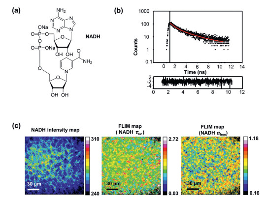
To analyze the metabolic state of brain tissues at high resolution, we set up a two-photon fluorescence lifetime imaging platform. The accessories and a simple optical path diagram of this platform are shown in Fig. S1 (Supporting information). The chemical formula for NADH is shown in Fig. 1a. NADH in fixed cerebral slice samples was excited with a two-photon 740 nm excitation laser, and the emissions were recorded using a 466/40-nm bandpass filter. Finally, in each image pixel, the fluorescence decay data were analysed using a two-component exponential fitting model (Fig. 1b), which produced images of the lifetime of the free NADH (τfree), the lifetime of the bound NADH lifetime (τbound), average lifetime (τav), and free and bound NADH amplitude weighting factors (αfree and αbound), as shown in Fig. 1c and the supporting information. Pertinently, αfree and αbound represent the free and bound NADH fractions respectively.
Figure 1
Figure 1.
Two-photon NADH FLIM of mouse cerebral nuclei in PFA-fixed slices. (a) Chemical formula for NADH. (b) The attenuation data of photons were fitted to an assumed attenuation model using software (Vistavision, ISS). (c) The NADH intensity map, fluorescence average lifetime (τav) map and αfree map were calculated by Vistavision, providing metabolic information on mouse cerebral nuclei.
In contrast to epidermal and cortical tissue, cerebral nuclei are too deep for in vivo imaging. Therefore, PFA-fixed mouse cerebral slices [26, 27] were chosen for NADH FLIM analysis to provide high resolution images and to obtain information about the metabolic state of cerebral nuclei at a specific time point. Mice were kept for one week in standard 12 h light/12 h dark entrainment conditions (lights on at 8:00 am, lights off at 8:00 pm) with ad libitum access to food, water, and running wheels. Their locomotor activity was monitored to ensure that the mice had a stable rhythm (Fig. S2 in Supporting information). All animal procedures were approved by the Institutional Animal Care and Use Committees of the University of Science and Technology of China (USTC) and the Chinese Academy of Sciences (CAS).
Then, we anaesthetized each mouse at a certain time point and took the brain for cryotome slicing after paraformaldehyde perfusion fixation and sucrose dehydration. To ensure that the two-photon FLIM of NADH can reflect the metabolic state of cerebral nuclei effectively at high resolution, we first examined the feasibility and stability of the PFA fixed slice metabolic imaging results using the two-photon FLIM platform.
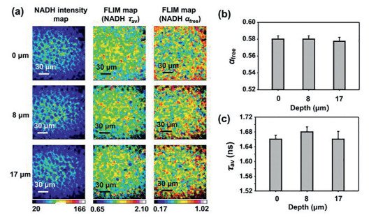
Initially, the easily identifiable dentate gyrus (DG) areas of hippocampal slices were used for experiments. The top cell layer of the cerebral slice was defined as 0 µm. We performed two-photon FLIM of NADH on DG at 0 µm, 8 µm and 17 µm in the 150 µm × 150 µm square area that covered most of the DG, as the interval was roughly the thickness of a layer of cells. The intensity map and FLIM map of NADH average lifetime τav and free NADH fraction αfree are shown in Fig. 2a. More concisely, the average value of the free NADH fraction at different depths was almost the same as that shown in Fig. 2b, as well as the average lifetime τav shown in Fig. 2c. Therefore, fine-tuning the focal length during the operation would not affect the fitting result.
Figure 2
Figure 2.
Two-photon NADH FLIM of the mouse DG at different depths. (a) NADH intensity map, NADH average tau (τav) map and αfree map of DG at 0 µm, 8 µm and 17 µm. (b) The mean values of αfree at different depths were approximately the same (0 µm: 0.5800 ± 0.008, 8 µm: 0.5800 ± 0.008, 17 µm: 0.5775 ± 0.01; P > 0.05, there were no significant differences among the 3 groups, one-way ANOVA, n = 4). (c) The mean values of the NADH average tau (τav) at different depths were almost the same (0 µm: 1.66 ± 0.022, 8 µm: 1.68 ± 0.027, 17 µm: 1.66 ± 0.042; P > 0.05, there were no significant differences among the 3 groups, one-way ANOVA, n = 4).
Since a 40 × objective may not cover the whole SCN, we performed two-photon FLIM on 5 different areas of the SCN (150 µm × 150 µm each area) in one slice sample (Figs. S3a and c in Supporting information). We found a series of similar values of free NADH fractions αfree (Fig. S3d in Supporting information). Because the consistency of the depth of cerebral slices in the SCN for each mouse cannot be guaranteed every time, we then tested the FLIM of selective areas in the SCN on 4 adjacent slices. The metabolic levels of the SCN region on the 4 adjacent slices were also similar to those of αfree (Figs. S3b and e in Supporting information). These results showed that the metabolic profile of the whole SCN in this experiment was almost the same.
We also examined the metabolic levels of three other nuclei, namely, the paraventricular nucleus of the hypothalamus (PVN), corpus callosum (CC) and caudate putamen (CPu), in the same cerebral slice. The results showed that the metabolic level of the PVN was similar to that of the SCN, whereas the CC and CPU were significantly different (Fig. S4 in Supporting information). Therefore, high-resolution metabolic state imaging using two-photon FLIM on mouse cerebral slices demonstrated high stability and reproducibility.
Because of the previously established relationship between the SCN and the circadian rhythm, we wondered whether the circadian rhythm controls cell metabolism in cerebral nuclei. Therefore, we applied two-photon FLIM of NADH to the SCN to investigate metabolic changes within a day. Six time points (10:00 am, 2:00 pm and 6:00 pm as daytime measurement points and 10:00 pm, 2:00 am, and 6:00 am as nighttime measurement points) were chosen for preparation of cerebral slice samples, and the experiments were repeated four times with different mice.
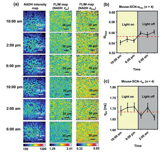
For each mouse, 4 adjacent slices and 8 different SCN regions were scanned using two-photon FLIM of NADH. The results showed that αfree and the average lifetime τav of the SCN oscillate within a day. In addition, αfree displayed a relatively stable level in the daytime (10:00 am, 2:00 pm and 6:00 pm), while two hours after the light was turned off, αfree showed an acute increase and then decreased and increased for the next ten hours, suggesting an ultradian oscillation of αfree at night. Receiving the light-off signal, the cells in the SCN entered an acute reaction state, with a relatively higher glycolysis level than that in the daytime. This high glycolysis level might not have lasted for a long time; a drop occurred later, and then the glycolysis level returned. Meanwhile, the average lifetime τav showed an opposite oscillation trend since the average lifetime τav is inversely proportional to αfree (Fig. 3). This metabolic rhythm might be involved in the SCN-related circadian rhythm.
Figure 3
Figure 3.
Two-photon NADH FLIM of the SCN at six time points within a day. (a) NADH intensity map, NADH average tau (τav) map and αfree map of the SCN at six time points within a day. (b) The mean value of αfree on the SCN displayed a circadian rhythm within a day. (c) The average lifetime τav in the SCN displayed a circadian rhythm within a day.
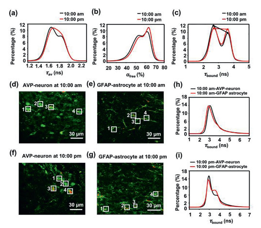
Considering the influence of different bound proteins on the NADH lifetime, we further drew the distribution of the average lifetimes τav, αfree and τbound of the SCN at 10:00 am and 10:00 pm using high-resolution analysis (Figs. 4a-c), representing early daytime and early night, respectively. Two main peaks can be distinguished in all three distributions. For the average lifetime τav and αfree (Figs. 4a and b), the two peaks might represent at least two groups of cells with different metabolic levels in the SCN. When comparing the average lifetime τav and αfree at 10:00 am with that at 10:00 pm, an obvious shift can be observed, suggesting that the metabolic oscillation of the SCN might be due to the change in the metabolism level of different tissue regions. Additionally, there were two peaks in the τbound distribution (Fig. 4c), suggesting that the proteins that bind to NADH might be divided into at least two major groups differ in their resultant shift in the NADH lifetime. The proportion of these two peaks changed between the 10:00 am and 10:00 pm recordings, leading to an in-depth study of the influence of NADH-binding proteins in different cell types on the metabolic oscillations of the cerebral nuclei.
Figure 4
Figure 4.
The distribution of NADH average tau (a), αfree (b) and τbound (c) using high-resolution analysis were compared at 10:00 am and 10:00 pm and two-photon NADH FLIM of Alexa647-labelled AVP-neurons and GFAP-astrocytes at 10:00 am and 10:00 pm. (d) Two-photon Alexa647 fluorescence imaging at 10:00 am of AVP-neurons labelled with Alexa647 by immunostaining. (e) Two-photon Alexa647 fluorescence imaging at 10:00 am of GFAP-astrocytes labelled with Alexa647 by immunostainin. (f) Two-photon Alexa647 fluorescence imaging at 10:00 pm of AVP-neurons labelled with Alexa647 by immunostaining. (g) Two-photon Alexa647 fluorescence imaging at 10:00 pm of GFAP-astrocytes labelled with Alexa647 by immunostaining. (h, i) The distribution of the τbound difference between AVP-neurons and GFAP-astrocytes at 10:00 am and 10:00 pm displaying no significant difference between AVP-neurons and GFAP-astrocytes at 10:00 am but a dramatic difference at 10:00 pm.
To ascertain the influence of different cell types on metabolic state oscillations, we tested two typical cell types in the SCN: neurons and glial cells. Arginine vasopressin (AVP)-positive neurons, a neuron type that expresses AVP, constitutes the largest population of SCN neurons. Glial cells are present in quantities 10–50 times the number of neurons in the SCN, while astrocytes are the most abundant cell type, which express glial fibrillary acidic protein (GFAP) [33]. Here, AVP-positive neurons (hereafter referred to as AVP-neurons) and GFAP-positive astrocytes (hereafter referred to as GFAP-astrocytes) in mouse cerebral slices at 10:00 am or 10:00 pm were labelled with Alexa Fluor 647 by immunostaining. Then, the fluorescence of Alexa Fluor647 was detected to locate the specific cell type (Figs. 4d-g) for subsequent two-photon FLIM of NADH. For each mouse, 8 adjacent slices were divided into two groups for immunostaining, and 16 cells from each group were selected for testing. Immunostaining was carefully performed simultaneously to reduce systematic error. At 10:00 am, the αfree of GFAP-astrocytes showed no significant difference from that of AVP-neurons (Fig. S5 in Supporting information), suggesting these two cell types have similar metabolic levels in the daytime. At 10:00 pm, the αfree of GFAP-astrocytes was significantly higher than that of AVP-neurons (Fig. S5), indicating that GFAP-astrocytes preferred glycolysis over oxidative phosphorylation more than AVP-neurons at early nighttime compared with early daytime.
Furthermore, we compared the distribution of τbound between 10:00 am and 10:00 pm. At 10:00 am, the distribution of τbound in either GFAP-astrocytes or AVP-neurons exhibited one obvious peak, with a very slight shift (Fig. 4h, Fig. S6 in Supporting information), suggesting that the influence of the binding protein on the NADH lifetime was similar in these two cell types in the daytime. At 10:00 pm, there were two significant peaks in the distribution of τbound in both AVP-neurons and GFAP-astrocytes. More interestingly, the second peak was significantly higher in GFAP-astrocytes than in AVP-neurons (Fig. 4i), and the absolute difference in peak 2/peak 1 between GFAP-astrocytes and AVP-neurons was 10 times that at 10:00 am (Fig. S7 in Supporting information), indicating that the protein that binds to NADH in GFAP-astrocytes was dramatically changed at the onset of night compared with that of daytime. Hence, the protein types that bind to NADH as well as the preference of the metabolic pathway of astrocytes might be the most important reasons for SCN metabolism oscillation. It has been reported in the literature that, compared with neurons, glial cells favor glycolysis rather than oxidation phosphorylation [34, 35].
Therefore, the two-photon NADH FLIM method provided high resolution images, but similar results were obtained by established destructive methods. More importantly, NADH FLIM pointed out the involvement of different cell types and NADH-bound proteins in the metabolic state oscillation of the SCN in the deep region of the brain. This work illustrates the feasibility and stability of two-photon FLIM of NADH on fixed mouse cerebral slices. Combining high-resolution imaging and immunostaining, we demonstrated at high resolution that the metabolic state variation and protein binding status of NADH in the two main cell types might be an important reason for cerebral metabolic state oscillation.
Due to the low resolution, external labeling requirement and destructiveness of traditional metabolic imaging methods, it was difficult to obtain high-resolution cell-level metabolic images of deep regions in the mouse brain. Therefore, two-photon FLIM of NADH of PFA-fixed cerebral slices is a potential imaging method to capture metabolic activity. Furthermore, clinical samples are usually preserved by chemical fixation for morphological stabilization of tissue, and chemical fixation is especially essential for enzymatic and histopathology studies. Therefore, fixed samples not only eliminate the effects of long-term anesthesia on cell metabolism in metabolism imaging in vivo but also provide the convenience and possibility of metabolism imaging of samples from the clinic.
Therefore, the two-photon NADH FLIM method can make full use of clinical samples and enable imaging of deep brain areas. More importantly, the results of this work enrich the present knowledge regarding the role of the metabolic properties of neurons and glial cells as well as the protein binding status of NADH in metabolic oscillation of cerebral nuclei, providing a high-resolution, sensitive and label-free method to explore metabolism and cell type classification in deep brain regions.
Declaration of competing interest
The authors declare that they have no known competing financial interests or personal relationships that could have appeared to influence the work reported in this paper.
Acknowledgments
This work was supported by the National Key R & D Program of China (Nos. 2016YFA0400900 and 2017YFA0505301), and National Natural Science Foundation of China (No. U1832181).
Supplementary materials
Supplementary material associated with this article can be found, in the online version, at doi:10.1016/j.cclet.2022.04.058.
R. Mostany, A. Miquelajauregui, M. Shtrahman, C. Portera-Cailliau, Two-Photon Excitation Microscopy and Its Applications in Neuroscience, in: P.J. Verveer (Ed. ), Advanced Fluorescence Microscopy: Methods and Protocols, Eds., Springer Science Business Media, New York, 2015, pp. 25–42.
[14]
B. Belardi, A.D.L. Zerda, D.R. Spiciarich, et al., Angew. Chem. Int. Ed. 52 (2013) 14045–14049. doi: 10.1002/anie.201307512
[15]
A. Bhattacharjee, R. Datta, E. Gratton, A.I. Hochbaum, Sci. Rep. 7 (2017) 3743. doi: 10.1038/s41598-017-04032-w
[16]
L.P. Bernier, E.M. York, A. Kamyabi, et al., Nat. Commun. 11 (2020) 1559. doi: 10.1038/s41467-020-15267-z
R. Mongeon, V. Venkatachalam, G. Yellen, Antioxid. Redox. Sign. 25 (2016) 553–563. doi: 10.1089/ars.2015.6593
Figure 1
Two-photon NADH FLIM of mouse cerebral nuclei in PFA-fixed slices. (a) Chemical formula for NADH. (b) The attenuation data of photons were fitted to an assumed attenuation model using software (Vistavision, ISS). (c) The NADH intensity map, fluorescence average lifetime (τav) map and αfree map were calculated by Vistavision, providing metabolic information on mouse cerebral nuclei.
Figure 2
Two-photon NADH FLIM of the mouse DG at different depths. (a) NADH intensity map, NADH average tau (τav) map and αfree map of DG at 0 µm, 8 µm and 17 µm. (b) The mean values of αfree at different depths were approximately the same (0 µm: 0.5800 ± 0.008, 8 µm: 0.5800 ± 0.008, 17 µm: 0.5775 ± 0.01; P > 0.05, there were no significant differences among the 3 groups, one-way ANOVA, n = 4). (c) The mean values of the NADH average tau (τav) at different depths were almost the same (0 µm: 1.66 ± 0.022, 8 µm: 1.68 ± 0.027, 17 µm: 1.66 ± 0.042; P > 0.05, there were no significant differences among the 3 groups, one-way ANOVA, n = 4).
Figure 3
Two-photon NADH FLIM of the SCN at six time points within a day. (a) NADH intensity map, NADH average tau (τav) map and αfree map of the SCN at six time points within a day. (b) The mean value of αfree on the SCN displayed a circadian rhythm within a day. (c) The average lifetime τav in the SCN displayed a circadian rhythm within a day.
Figure 4
The distribution of NADH average tau (a), αfree (b) and τbound (c) using high-resolution analysis were compared at 10:00 am and 10:00 pm and two-photon NADH FLIM of Alexa647-labelled AVP-neurons and GFAP-astrocytes at 10:00 am and 10:00 pm. (d) Two-photon Alexa647 fluorescence imaging at 10:00 am of AVP-neurons labelled with Alexa647 by immunostaining. (e) Two-photon Alexa647 fluorescence imaging at 10:00 am of GFAP-astrocytes labelled with Alexa647 by immunostainin. (f) Two-photon Alexa647 fluorescence imaging at 10:00 pm of AVP-neurons labelled with Alexa647 by immunostaining. (g) Two-photon Alexa647 fluorescence imaging at 10:00 pm of GFAP-astrocytes labelled with Alexa647 by immunostaining. (h, i) The distribution of the τbound difference between AVP-neurons and GFAP-astrocytes at 10:00 am and 10:00 pm displaying no significant difference between AVP-neurons and GFAP-astrocytes at 10:00 am but a dramatic difference at 10:00 pm.

 DownLoad:

 下载:
下载: